Visualization

This tutorial demonstrates interactive visualization with solvation_analysis and nglview. NGLview creates interactive widgets that can be manipulated in Jupyter notebooks. You are encouraged to set up NGLview locally so that you can explore this yourself. For those who can’t, static images of the output will be shown.

# imports
import MDAnalysis as mda
from solvation_analysis.solute import Solute
from solvation_analysis.tests import datafiles

from IPython.display import Image

# instantiate Universe
u = mda.Universe(datafiles.ea_fec_pdb, datafiles.ea_fec_dcd)

The setup here should be familiar. We define all of our atom groups of interest and use them to instantiate a solution. EA and FEC have similar compositions so we select them by slicing the array of residues.

# define solute AtomGroup
li_atoms = u.atoms.select_atoms("element Li")

# define solvent AtomGroups
EA = u.residues[0:235].atoms                    # ethyl acetate
FEC = u.residues[235:600].atoms                 # fluorinated ethylene carbonate
PF6 = u.atoms.select_atoms("byres element P")   # hexafluorophosphate

# instantiate solution
solute = Solute.from_atoms(li_atoms,
                    {'EA': EA, 'FEC': FEC, 'PF6': PF6},
                    radii={'PF6': 2.6, 'FEC': 2.7})

solute.run()

<solvation_analysis.solute.Solute at 0x7f8028cda160>

Primer on Nglview

nglview is a powerful interactive molecular visualization package. Unfortunately, it can be a bit of hassle to get working properly. Make sure you have ipywidgets installed before working with nglview.

For more information on nglview, check out their website or the MDAnalysis nglview tutorial.

The cell below provides a test case for your Jupyter notebook configuration. If everything is configured properly, the cell will print a rectangle with “Hello, World” printed inside. If your Jupyter environment is configured incorrectly, it will instead print Text(value='Hello, World').

# import nglview
import nglview as nv

# test Jupyter configuration
from ipywidgets import Text
Text("Hello, World")

Visualizing the Trajectory

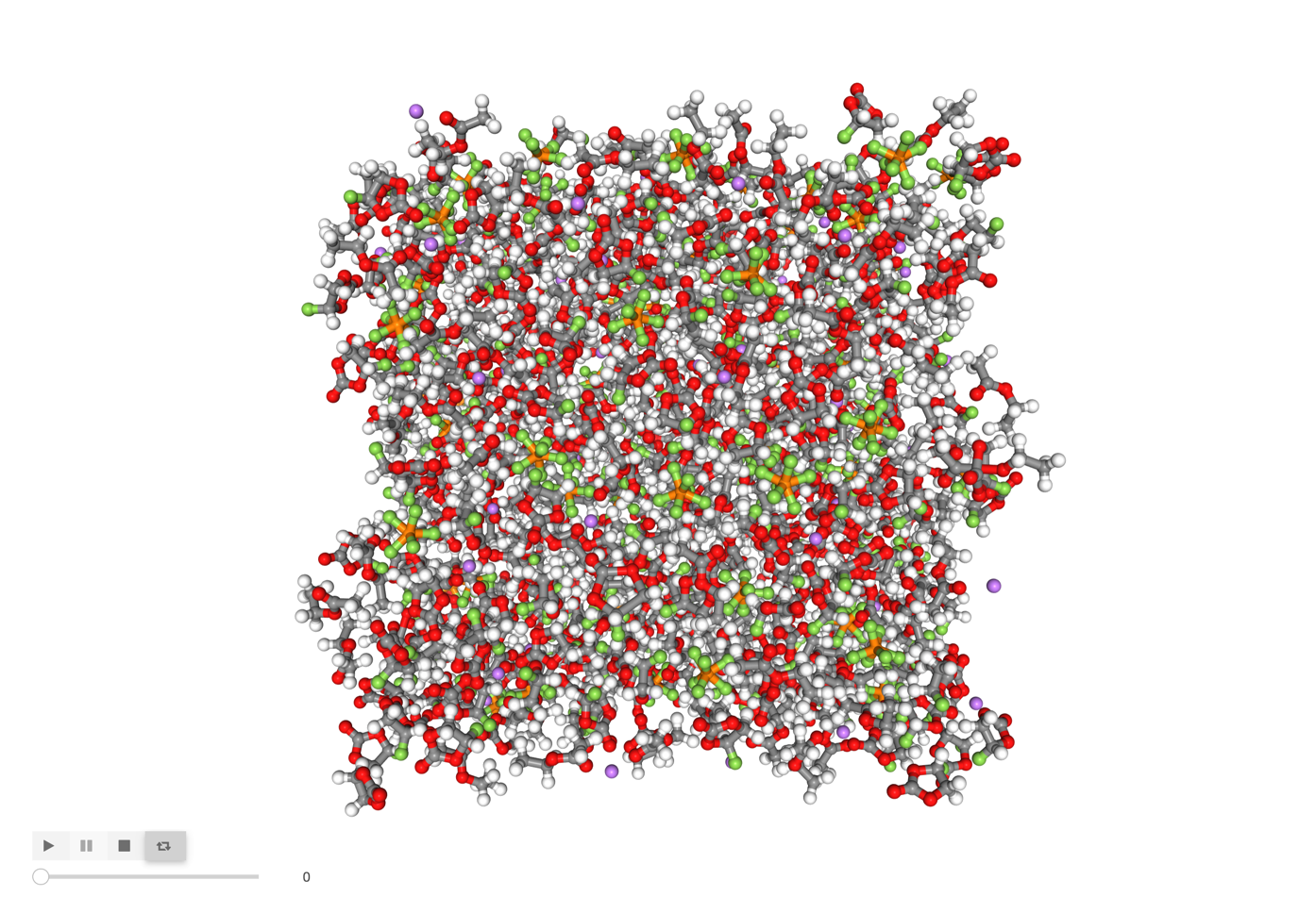
Now the exciting part, visualizing! We will start with a simple visualization of all atoms.

First, we call nv.show_mdanalysis() on an AtomGroup to instantiate an mda_view, which contains a persistent view of an MDA AtomGroup. Next, we call mda_view.display() to visualize our trajectory below the cell.

If you are executing this in a jupyter notebook, the following cell should display a interactive NGLView widget. Since this will not render in the online tutorial, the next cell includes an image of what the cell WOULD output. We’ll include both cells for all following visualizations.

mda_view = nv.show_mdanalysis(u.atoms)
mda_view.display()

# this is what you should see
Image('images/all_atoms.png', width=600)

For convenience, I recommend wrapping this into a one-liner function, shown below. This is how we will use nglview for the remainder of the tutorial.

def visualize(atom_group):
    mda_view = nv.show_mdanalysis(atom_group)
    return mda_view.display()

Interactive visualization

To kick off the interactive visualization workflow, we need to find something we are interested in visualizing! Let’s see which atoms EA, FEC, and PF66- tend to coordinate with. We will start with EA.

First lets see which EA solvation shell composition is most common.

# return the percentage of each shell
solute.speciation.speciation_fraction.head()

	EA	FEC	PF6	count
0	3	1	0	0.252459
1	2	3	0	0.173770
2	2	2	0	0.132787
3	1	3	0	0.086885
4	4	0	0	0.059016

Looks like 3 EA and 1 FEC is the most common shell. Let’s find one to visualize!

# find all shells with 3 EA, 1 FEC, and 0 PF6
solute.speciation.get_shells({'EA': 3, 'FEC': 1, 'PF6': 0}).head()

	solvent	EA	FEC	PF6
frame	solute_ix
0	603	3	1	0
	610	3	1	0
	616	3	1	0
	620	3	1	0
	621	3	1	0

Let’s go with the top, solute 603 in the frame 0. We’ll save the AtomGroup as shell. Just to be safe we’ll print the shell DataFrame to make sure we have the right composition.

# save the AtomGroup
shell = solute.get_shell(solute_index=603, frame=0)

# print the DataFrame
solute.get_shell(603, 0, as_df=True)

		distance	solute	solvent	solvent_ix
solute_atom_ix	solvent_atom_ix
6943	2315	1.943975	solute_0	EA	165
	1223	1.997783	solute_0	EA	87
	3141	2.054177	solute_0	EA	224
	3320	2.265687	solute_0	FEC	238

Looks good! Now we are ready to take a look.

visualize(shell)

Image('images/shell.png', width=600)

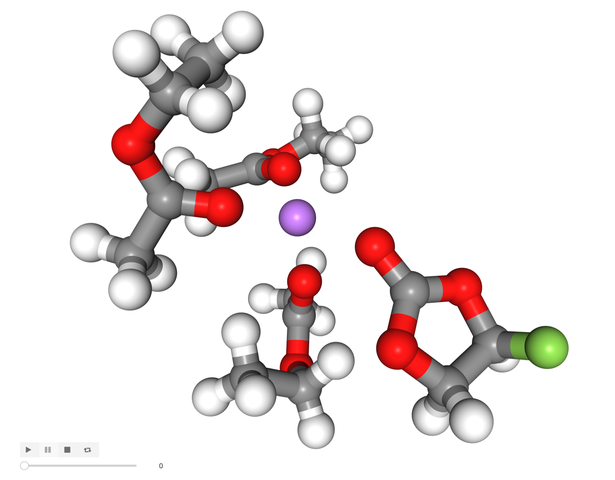
Easy! Let’s explore further.

There appears to be an uncoordinated molecule to one side of our Li ion, lets investigate with the get_closest_n_mol selection function.

u.trajectory[0]
shell_5 = solute.get_closest_n_mol(solute_atom_ix=6943, n_mol=5)

visualize(shell_5)

Image('images/shell_5.png', width=600)

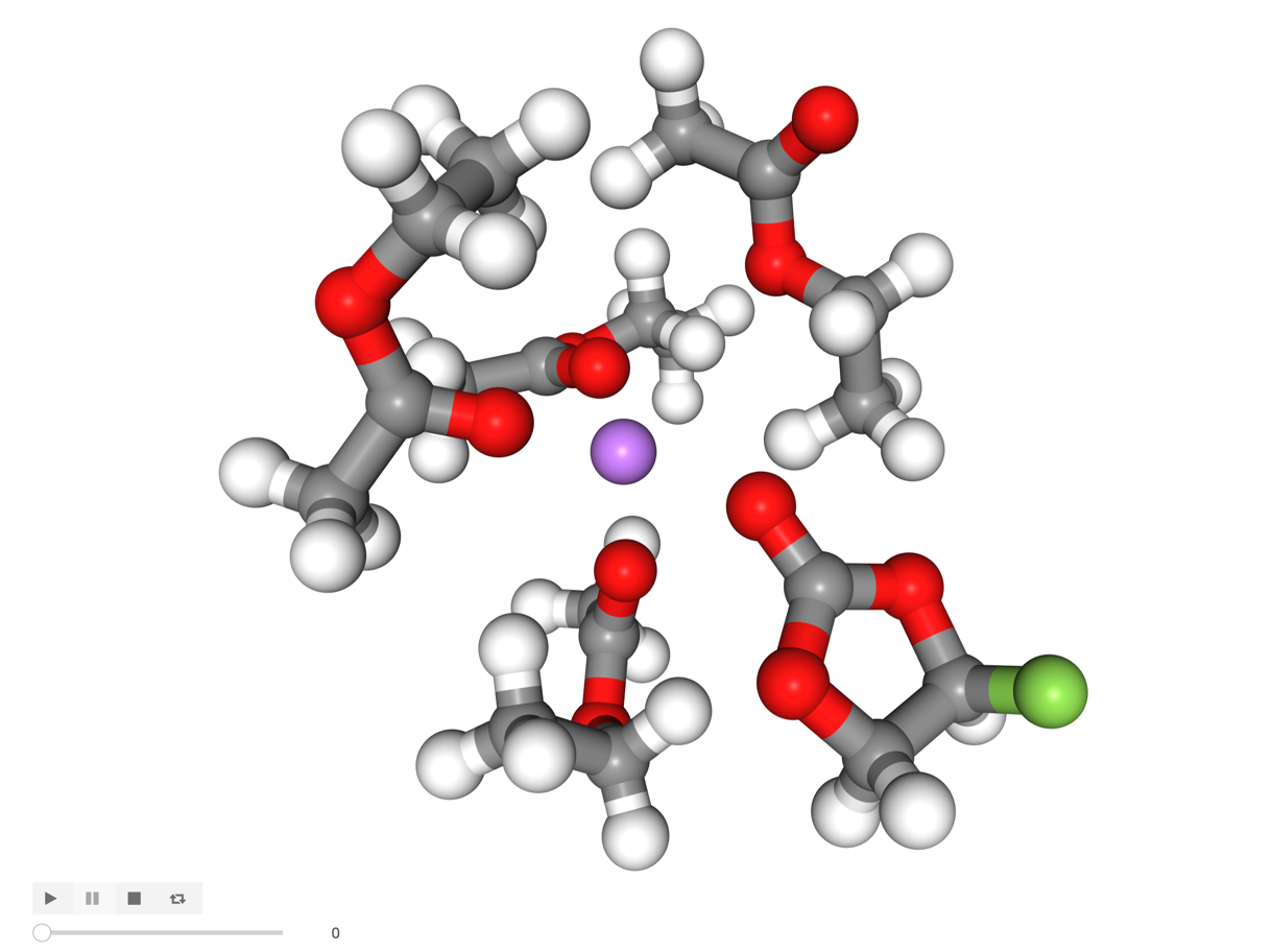
An uncoordinated EA molecule is there but it’s not oriented correctly to coordinate with its carbonyl oxygen.

We’ll stop there, but hopefully this provides a taste of what interactive visualization can look like!