Residence and Networking
Solute setup is covered in detail in the basics_tutorial so it will not be covered here.
If you are new to solvation_analysis check there first!
[1]:
# imports
import MDAnalysis as mda
from solvation_analysis import Solute

# we will use a trajectory supplied by the package
from solvation_analysis.tests import datafiles

# instantiate Universe
u = mda.Universe(datafiles.bn_fec_data, datafiles.bn_fec_dcd_unwrap)

# define solute AtomGroup
li_atoms = u.atoms.select_atoms("type 22")

# define solvent AtomGroups
PF6 = u.atoms.select_atoms("byres type 21")
BN = u.atoms.select_atoms("byres type 5")
FEC = u.atoms.select_atoms("byres type 19")

solute = Solute.from_atoms(li_atoms, {'PF6': PF6, 'BN': BN, 'FEC': FEC}, radii={'PF6': 2.6})

solute.run()
Warning: importing 'simtk.openmm' is deprecated. Import 'openmm' instead.
[1]:
<solvation_analysis.solute.Solute at 0x7feaa88c3fd0>
We will be covering the Residence and Networking analysis objects. Though these are easy to instantiate and use, they are not instantiated by default because they can be expensive.
We’ll start with Residence, which we will instantiate with the from_solute method.
Calculating Residence Times
[2]:
from solvation_analysis.residence import Residence

# warnings are expected
residence = Residence.from_solute(solute)
/Users/orioncohen/miniconda3/envs/solvation_analysis/lib/python3.8/site-packages/pandas/core/apply.py:131: FutureWarning: the 'unbiased'' keyword is deprecated, use 'adjusted' instead
  return func(x, *args, **kwargs)
/Users/orioncohen/projects/development/solvation-analysis/solvation-analysis/solvation_analysis/residence.py:148: UserWarning: the autocovariance for BN does not converge to zero so a residence time cannot be calculated. A longer simulation is required to get a valid estimate of the residence time.
  warnings.warn(f'the autocovariance for {res_name} does not converge to zero '
/Users/orioncohen/projects/development/solvation-analysis/solvation-analysis/solvation_analysis/residence.py:148: UserWarning: the autocovariance for FEC does not converge to zero so a residence time cannot be calculated. A longer simulation is required to get a valid estimate of the residence time.
  warnings.warn(f'the autocovariance for {res_name} does not converge to zero '
/Users/orioncohen/projects/development/solvation-analysis/solvation-analysis/solvation_analysis/residence.py:148: UserWarning: the autocovariance for PF6 does not converge to zero so a residence time cannot be calculated. A longer simulation is required to get a valid estimate of the residence time.
  warnings.warn(f'the autocovariance for {res_name} does not converge to zero '
Because we are only looking at a very short snapshot of the simulation, the residence times here are NOT physically meaningful. That’s why we get so many warnings. For the sake of the tutorial, let’s imagine that we had a long enough simulation to get good results.
Residence automatically calculates the residence times of all the solvents with either with either a “cutoff” method or a “fit” method. The documentation of Residence has more detail, but in brief, fit is more accurate and cutoff is less prone to convergence issues.
[3]:
# these will strongly disagree because our simulation time is too short
print("The cutoff residence times are: ", residence.residence_times_cutoff)
print("The fit residence times are:    ", residence.residence_times_fit)
The cutoff residence times are:  {'BN': nan, 'FEC': 6, 'PF6': 9}
The fit residence times are:     {'BN': 4.63, 'FEC': 2.88, 'PF6': 1.15}
We have two methods for binding the Residence object to our Solute object. We can “monkey patch” our residence object directly into Solute.
[4]:
solute.residence = residence
solute.residence
[4]:
<solvation_analysis.residence.Residence at 0x7fea8840f8e0>
Or we can instantiate our Solute with the Residence object included, shown below.
This dichotomy of monkey-patching with from_solution vs specifying in the analysis_classes keyword applies to all the analysis classes in solvation-analyis.
[5]:
solute = Solute.from_atoms(
    li_atoms,
    {'PF6': PF6, 'BN': BN, 'FEC': FEC},
    radii={'PF6': 2.6},
    analysis_classes=["pairing", "coordination", "speciation", "residence"],
)
solute.run()
[5]:
<solvation_analysis.solute.Solute at 0x7fea483b2b50>
Networking follows an identical setup pattern except we specify which solvents should participate in the network. For example, in the example below we are interested in the network of cations and anions in a battery electrolyte. It doesn’t make sense to include the solvents in the network, so we choose to only look at networking with the anion.
Parsing Network Structure
[6]:
from solvation_analysis.networking import Networking

networking = Networking.from_solute(solute, 'PF6')
Now that we have the network, lets examine the core data structure of the Networking object.
[7]:
networking.network_df
[7]:
| solvent | solvent_ix | ||
|---|---|---|---|
| frame | network | ||
| 0 | 0 | PF6 | 603 |
| 0 | solute_0 | 683 | |
| 0 | solute_0 | 690 | |
| 1 | PF6 | 616 | |
| 1 | solute_0 | 670 | |
| ... | ... | ... | ... |
| 9 | 1 | solute_0 | 693 |
| 2 | PF6 | 623 | |
| 2 | solute_0 | 664 | |
| 3 | PF6 | 648 | |
| 3 | solute_0 | 668 |
112 rows × 2 columns
The network_df includes all of the solutes coordinated with at least one solvent, if these coordinated solvents form a network, they are grouped together into a single item in the network column of the dataframe.
Here, we can see that in frame 0, our 0th network has two solutes and one PF6 solvent and our 1st network has one solute and one solvent.
The second column lists the residue indexes (from the MDAnalysis Universe) of each listed species.
Networking also calculates several convenient statistics, such as the clusters size distribution:
[8]:
networking.network_sizes
[8]:
| solvent | 2 | 3 |
|---|---|---|
| frame | ||
| 0 | 4 | 2 |
| 1 | 4 | 1 |
| 2 | 5 | 1 |
| 3 | 6 | 0 |
| 4 | 6 | 0 |
| 5 | 3 | 0 |
| 6 | 5 | 0 |
| 7 | 7 | 0 |
| 8 | 4 | 1 |
| 9 | 3 | 1 |
and the “solute status”, or whether the solute is uncoordinated, coordinated with a single solvent, or in a network.
[9]:
networking.solute_status
[9]:
{'isolated': 0.8918367346938776,
 'paired': 0.09591836734693877,
 'networked': 0.012244897959183671}
As before, we can instantiate a Networking object in the solution directly, but this time, we’ll need to specify the solvent(s) of interest in the networking_solvents kwarg.
[10]:
solute = Solute.from_atoms(
    li_atoms,
    {'PF6': PF6, 'BN': BN, 'FEC': FEC},
    radii={'PF6': 2.6},
    analysis_classes=["pairing", "coordination", "speciation", "networking"],
    networking_solvents='PF6'
)
solute.run()
[10]:
<solvation_analysis.solute.Solute at 0x7fea71500400>
Visualizing Networks
Finally, we can effectively integrate the networking object into a visualization workflow by using the residue indexes and to select the cluster’s AtomGroup. This example relies on understanding the content in the Visualization Tutorial.
For this, we’ll need to quickly spin up a different solution to use as an example.
[11]:
from solvation_analysis.tests import datafiles

# instantiate Universe
u = mda.Universe(datafiles.ea_fec_pdb, datafiles.ea_fec_dcd)

# define solute AtomGroup
li_atoms = u.atoms.select_atoms("element Li")

# define solvent AtomGroups
EA = u.residues[0:235].atoms                    # ethyl acetate
FEC = u.residues[235:600].atoms                 # fluorinated ethylene carbonate
PF6 = u.atoms.select_atoms("byres element P")   # hexafluorophosphate

# instantiate solute
solute2 = Solute.from_atoms(
    li_atoms,
    {'EA': EA, 'FEC': FEC, 'PF6': PF6},
    radii={'PF6': 2.6, 'FEC': 2.7},
    solute_name="Li",
    analysis_classes=["pairing", "coordination", "speciation", "networking"],
    networking_solvents=['PF6', 'FEC']
)

solute2.run()
[11]:
<solvation_analysis.solute.Solute at 0x7fea68f79490>
For the sake of getting a nice big cluster to visualize, we use both PF6 and FEC as networking solvents, this isn’t particularly interesting scientifically, but it’s nicer to look at!
[12]:
networking = solute2.networking
networking.network_df.head(32)
[12]:
| solvent | solvent_ix | ||
|---|---|---|---|
| frame | network | ||
| 0 | 0 | FEC | 236 |
| 0 | FEC | 245 | |
| 0 | Li | 653 | |
| 1 | FEC | 238 | |
| 1 | Li | 603 | |
| 2 | FEC | 239 | |
| 2 | FEC | 241 | |
| 2 | FEC | 533 | |
| 2 | Li | 660 | |
| 3 | FEC | 242 | |
| 3 | Li | 639 | |
| 4 | FEC | 243 | |
| 4 | FEC | 494 | |
| 4 | Li | 635 | |
| 5 | FEC | 244 | |
| 5 | FEC | 413 | |
| 5 | FEC | 580 | |
| 5 | Li | 609 | |
| 6 | FEC | 247 | |
| 6 | FEC | 264 | |
| 6 | FEC | 274 | |
| 6 | FEC | 381 | |
| 6 | FEC | 523 | |
| 6 | FEC | 540 | |
| 6 | FEC | 541 | |
| 6 | FEC | 573 | |
| 6 | Li | 612 | |
| 6 | Li | 631 | |
| 6 | Li | 658 | |
| 7 | FEC | 248 | |
| 7 | FEC | 306 | |
| 7 | FEC | 460 |
[13]:
# import nglview
import nglview as nv
from IPython.display import Image
def visualize(atom_group):
mda_view = nv.show_mdanalysis(atom_group)
return mda_view.display()
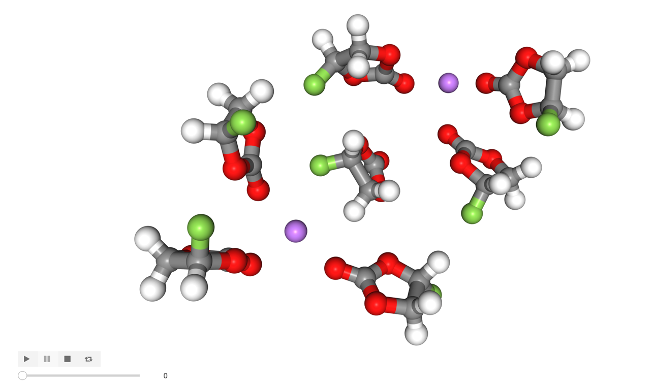
res_ix = networking.get_network_res_ix(6, 0)
network = solute2.u.residues[res_ix.astype(int)].atoms
visualize(network)
The network wraps around the periodic boundary so we can’t quite visualize it in one frame, but this is most of it:
[14]:
Image('images/network.png', width=600)
[14]:
Great! Now you should understand how to use both the Residence and Networking tools, for more detail, check out the documentation.